(1/N) ML Concepts - The Perceptron

This post borrows notation and structure from pages 18-57 of Anil Ananthaswamy’s fantastic book: “Why Machines Learn” (WML). Readers are expected to have some familiarity with concepts from Linear Algebra, including vectors, dot products, and related operations on vectors/matrices.

The Perceptron

The perceptron is a simple, ubiquitous, and conceptually important machine learning model and associated optimization algorithm. Essentially, it is a binary classifier that assigns samples, represented as points $\mathbf{x} \in \mathbb{R}^{1 \times d}$ to one of two categories $y \in \{-1, +1 \}$, and is parameterized by a weight vector $\mathbf{w} \in \mathbb{R}^{1 \times d}$ and a bias term $b \in \mathbb{R}$. Following conventions used in WML, we will write samples as $\mathbf{x} = [x_1, \dots, x_n]$ and weight vectors as $\mathbf{w} = [w_1, \dots, w_n]$. The Perceptron is remarkably compact; it can be expressed as a simple piecewise function:

\[y = \begin{cases} +1 & \sum_{i=1}^{n} w_i x_i + b \geq 0 \\ -1 & \text{otherwise} \end{cases} \text{.}\]

Or, using matrix multiplication instead of a weighted sum:

\[y = \begin{cases} +1 & \mathbf{w}^{\top} \mathbf{x} + b \geq 0 \\ -1 & \text{otherwise} \end{cases} \text{.}\]

Readers might also be familiar with the following, biologically-inspired diagram.

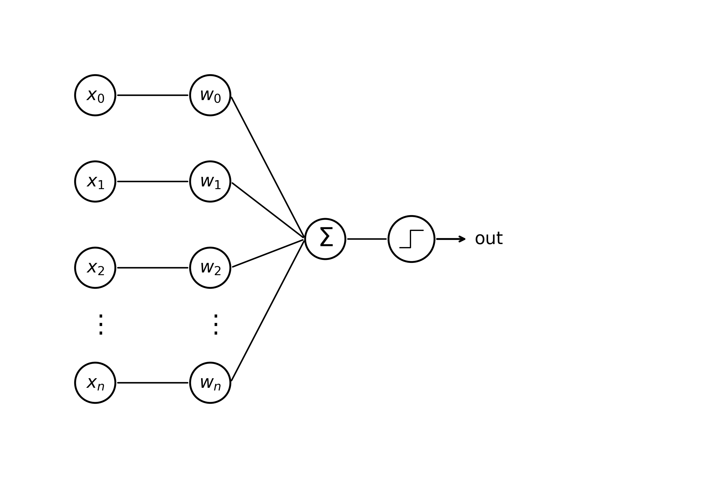
Weight edges connecting $x_i$ –> $w_i$ denote multiplication, edges from $w_i$ –> $\sum$ summation, and from $\sum$ –> (activation fn) thresholding. This machinery constitutes a single “neuron” of a neural network consisting of (1) incoming weights, (2) a bias term, and (3) a non-linear activation function. We can think of the equation above as characterizing a hyperplane with dimensionality $\mathbb{R}^{d - 1}$, capable of splitting any space in two. Points $\mathbf{x}$ that lie in $\mathbb{R}^{d}$ are classified as either $-1$ or $+1$ by our perceptron model. To make things more concrete, we’ll start off by showing the reader an example in $\mathbb{R}^{2}$ for a weight vector $\mathbf{w} = [1, 1]$ and bias term $b=0$.

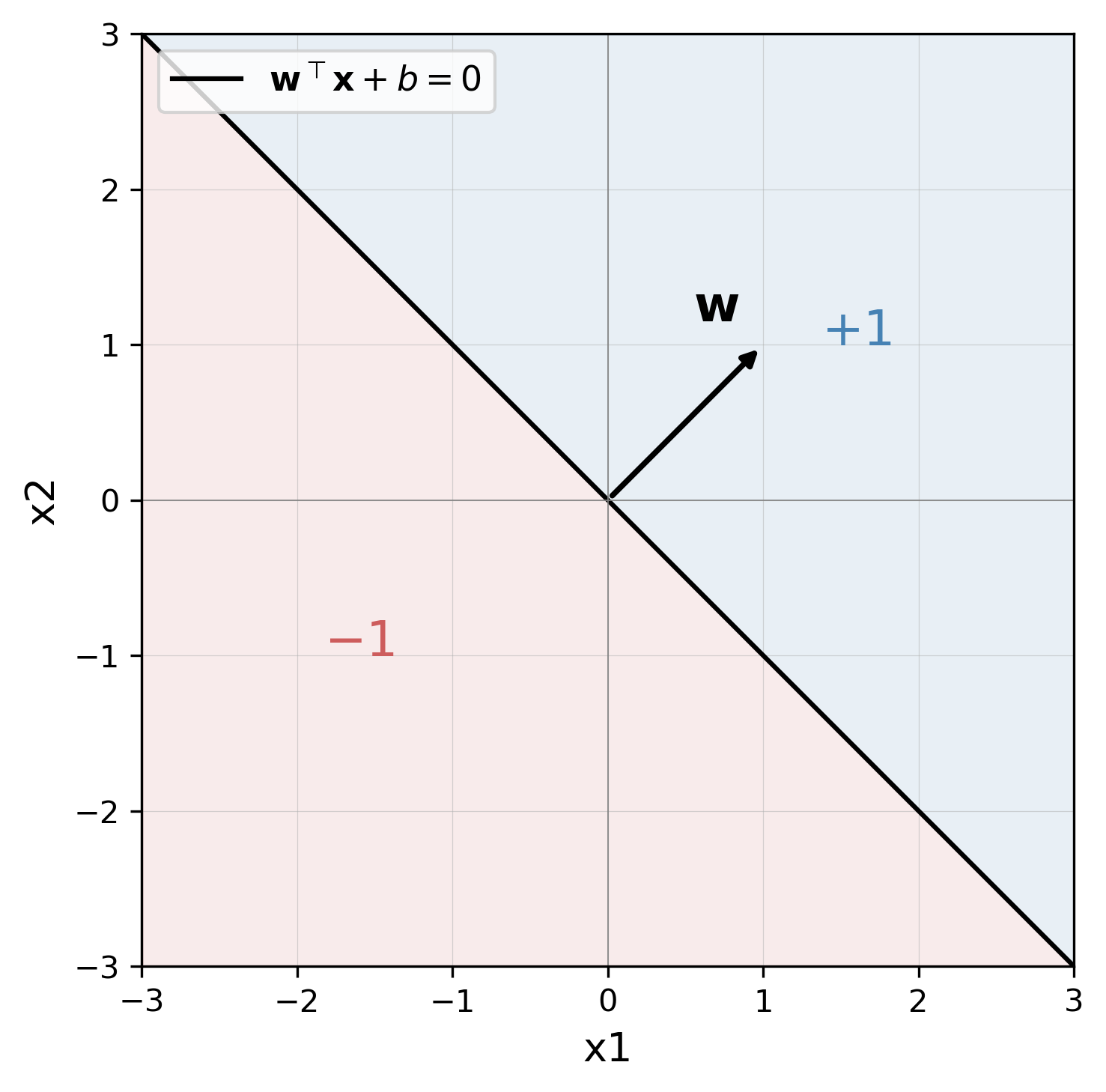
The weight vector $\mathbf{w}$, starting at the origin and extending toward $[1,1]$, is orthogonal to a plane of separation that passes through the origin when $b=0$. In this example, points that fall to the right of the black line are classified as $+1$, and points to the left as $-1$. It may seem straightforward, but what happens visually when we set the bias term to a non-zero value, say $b=-4$?

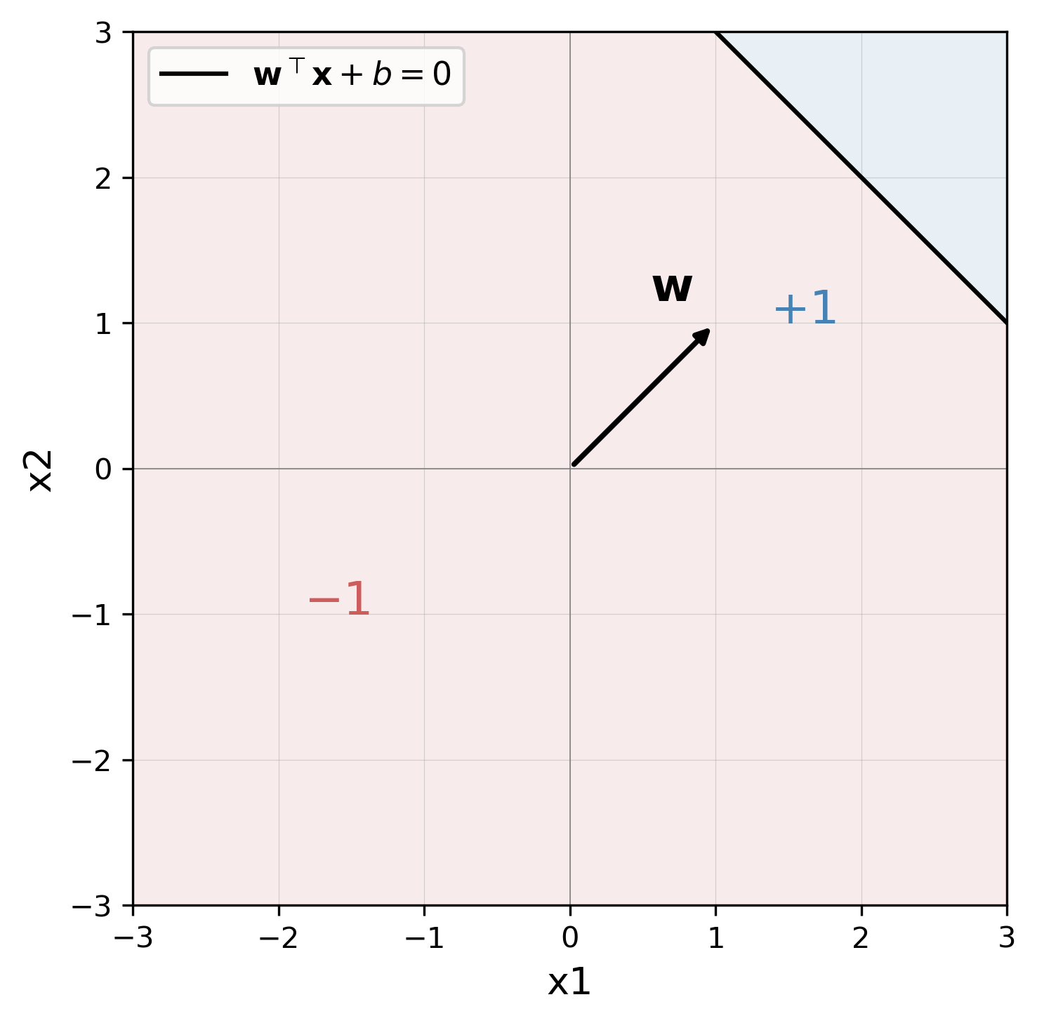
Our separating plane shifts toward the left, away from the origin. You can imagine that our weight vector $\mathbf{w}$ has been “translated” such that its magnitude remains the same, and its point of origin is $[-b, -b]$. This is just an intuition of course, and all vectors live at the origin. Now we can begin to turn our attention toward what the perceptron is actually good for: binary classification. Specifically, a perceptron can achieve perfect accuracy and generalization for any dataset whose points are linearly separable–that is, points belonging to different classes can be separated by a plane.

Consider a dataset of basketball players $\mathcal{D} = \{ (\mathbf{x}_i, y_i) \}_{i=1 \dots n}$, still in $\mathbb{R}^2$, where $\mathbf{x}_i = [\text{in. above avg. height}, \text{in. above avg. vertical leap}]$, and $y_i = +1$ and $y_i = -1$ indicate that player can or can not dunk, respectively. Reusing our perceptron model from earlier, our dataset might look like so:

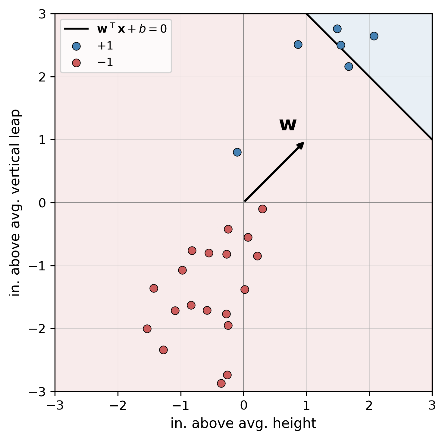
Yikes, it looks like our model has misclassified some dunkers as non-dunkers! Now we have a dilemma: we know that our dataset is linearly separable, but we don’t know how to set the values of $\mathbf{w}$ such that each sample is assigned to the correct class. This leads us to the Perceptron learning algorithm–a recursive procedure responsible for updating $\mathbf{w}$ and $b$ and which is guaranteed to succeed for any linearly separable dataset$^*$. We’ll start off by grouping the bias term $b$ into the weight matrix $\mathbf{w}$ for notational convenience. We can rewrite $\mathbf{x} = [x_0, x_1, \dots, x_n]$ and $\mathbf{w} = [w_0, w_1, \dots, w_n]$, where $x_0 = 1$ and $w_0 = b$. Note that while, in the example above, $\mathbf{x}$ and $\mathbf{w}$ now technically exist in $\mathbb{R}^3$, we can still visualize our perceptron in two-dimensions as before. Bias terms subsumed, our compacted model can be written as:

\[y = \begin{cases} +1 & \mathbf{w}^{\top} \mathbf{x} \geq 0 \\ -1 & \text{otherwise} \end{cases} \text{.}\]

Now we’re ready to define our optimization algorithm.

$$ \begin{aligned} &\textbf{Step 1: } \mathbf{w} \leftarrow \mathbf{0} \\ &\textbf{Step 2: } \text{for } \mathbf{x}_i \in \mathcal{D}\text{:} \\ &\quad \text{if } y_i \, \mathbf{w}^\top \mathbf{x}_i \leq 0\text{:} \\ &\quad\quad \mathbf{w} \leftarrow \mathbf{w} + y_i \, \mathbf{x}_i \\ &\textbf{Step 3: } \text{if no updates to } \mathbf{w} \text{ in Step 2: end} \\ &\quad \text{else: go to Step 2} \end{aligned} $$

At a high level, this procedure iterates through each point in our dataset. When we encounter a point that is misclassified, the algorithm updates $\mathbf{w}$ such that the plane of separation is “nudged” in the direction of the misclassified point. We repeat this process until every point is assigned to the correct label.

Miraculously, our work here is done! We have successfully defined and trained one of the essential models in modern AI with just a few concepts and lines of pseudo-code. While the Perceptron has some remarkable properties, namely a guarantee of convergence under the right conditions, a single neuron suffers some key limitations. First and foremost, how do we model datasets that can not be separated by a single plane? The answer is simple: we chain multiple neurons together into a “Multi-Layer Perceptron (MLP)!” But, these will have to wait until next week’s installment of ML Concepts.

Thanks for reading!

Footnotes

*A formal proof of this property is not included in this post; the reader is highly encouraged to view Prof. Kilian Weinberger’s lecture referenced below for a thorough treatment of this topic [1].

References

[1] Weinberger, K. (2017). Lecture 6 “Perceptron convergence proof”—Cornell CS4780 SP17 [Video]. YouTube. https://www.youtube.com/watch?v=kObhWlqIeD8
[2] Ananthaswamy, A. (2024). Why machines learn: The elegant math behind modern AI. Dutton.

The Perceptron

Footnotes

References

Enjoy Reading This Article?