(2/N) ML Concepts - The Multi-Layer Perceptron

This post makes use of notation and general concepts introduced in Chapter 4 of Christopher Bishop’s seminal textbook: “Neural Networks for Pattern Recognition.” Readers interested in building deeper intuition of the capabilities and limitations of neural networks–as well as the governing mathematics of machine learning–will benefit enormously from a review of this classic treatment.

The Multi-Layer Perceptron

Last week, we provided a brief overview of one of the basic building blocks of machine learning: the Perceptron. Specifically, we focused on the implementation of a single-unit Perceptron trained with an adaptive weight-update algorithm. Recall that this simple model is capable of classifying any linearly separable dataset, and can be defined using the following equation:

\[y = \begin{cases} +1 & \mathbf{w}^{\top} \mathbf{x} + b \geq 0 \\ -1 & \text{otherwise} \end{cases} \text{.}\]

But, what about the far more common, infinitely variable world of non-linearly separable datasets? What if, to accurately classify some dataset, we need to carve our input space into convex or even non-convex regions? To skillfully represent and extrapolate these data we will introduce a sequential function that (1) has learnable parameters that update based on observations, and (2) has some non-linearities baked in. To that end, today we are going to build a Multi-Layer Perceptron (MLP) bit by bit–slowly modifying our original Perceptron into a much more expressive model.

Let’s remember that a single-unit Perceptron can be thought of as a machine that maps input vector data \(\mathbf{x} \in \mathbb{R}^d\) to one of two outputs \(y \in \{ -1, +1\}\) via a weight vector \(\mathbf{w} \in \mathbb{R}^d\) and a bias term \(b\). Taken from another point of view, these mathematical operations can be visualized as the activation pattern for a single biological (albeit an anatomically incorrect) neuron. (For sake of elegance, we subsume the bias term \(b\) in the weight vector using a trick outlined in our previous ML concepts blog.)

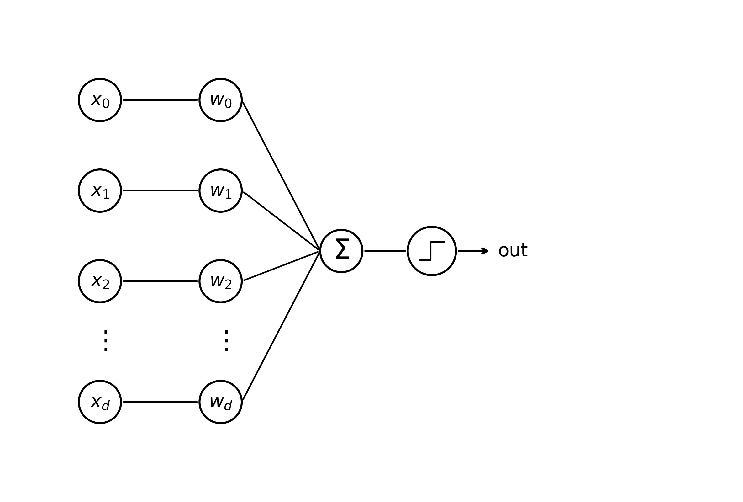
Here, edges connecting input values \(x_i\) to corresponding weights \(w_i\) represent multiplication.

Imagine instead that we wanted to map an input vector \(\mathbf{x}^{( \ell)}\) belonging to a network layer \(\ell\) not to a single, scalar output, but to another vector, call it \(\mathbf{a}^{( \ell + 1)} \in \mathbb{R}^M\). We could achieve this quite simply by replacing \(\mathbf{w}\) in the equation for a Perceptron with a weight matrix \(A \in \mathbb{R}^{d \times M}\), and calculating \(\mathbf{a}^{( \ell + 1)} = A^{\top}_{(\ell + 1)} \mathbf{x}^{( \ell )} + b_{(\ell + 1)}\). This linear transformation forms part of a “layer” of a modern neural network, and can be thought of as the input signal to a grouping of artificial “neurons”.

A non-linear activation function \(g(\cdot)\) is applied to obtain the final value of a hidden state vector \(\mathbf{z}^{(\ell + 1)} = g(\mathbf{a}^{( \ell + 1)})\). Once again, this added non-linearity is the secret sauce of deep learning; neural networks cannot learn non-linear mappings without non-linear activation functions, instead they degenerate into linear transforms that could be expressed as single-layer networks! Going back to the biological inspiration for MLPs, activation functions determine if, and how strongly, a particular neuron “fires”.

In practice, \(g(\cdot)\) can be implemented many different ways, and indeed different activation functions are used at different points in a neural network. Our Perceptron model used a version of the “Heaviside” step function (a simple binary threshold). When calculating intermediate activations \(\mathbf{z}\), today we will use the tanh function \(g \equiv \text{tanh}(a) = \frac{e^{a} - e^{-a}}{e^{a} + e^{-a}}\). A diagram of a single neural network layer can now be drawn like so.

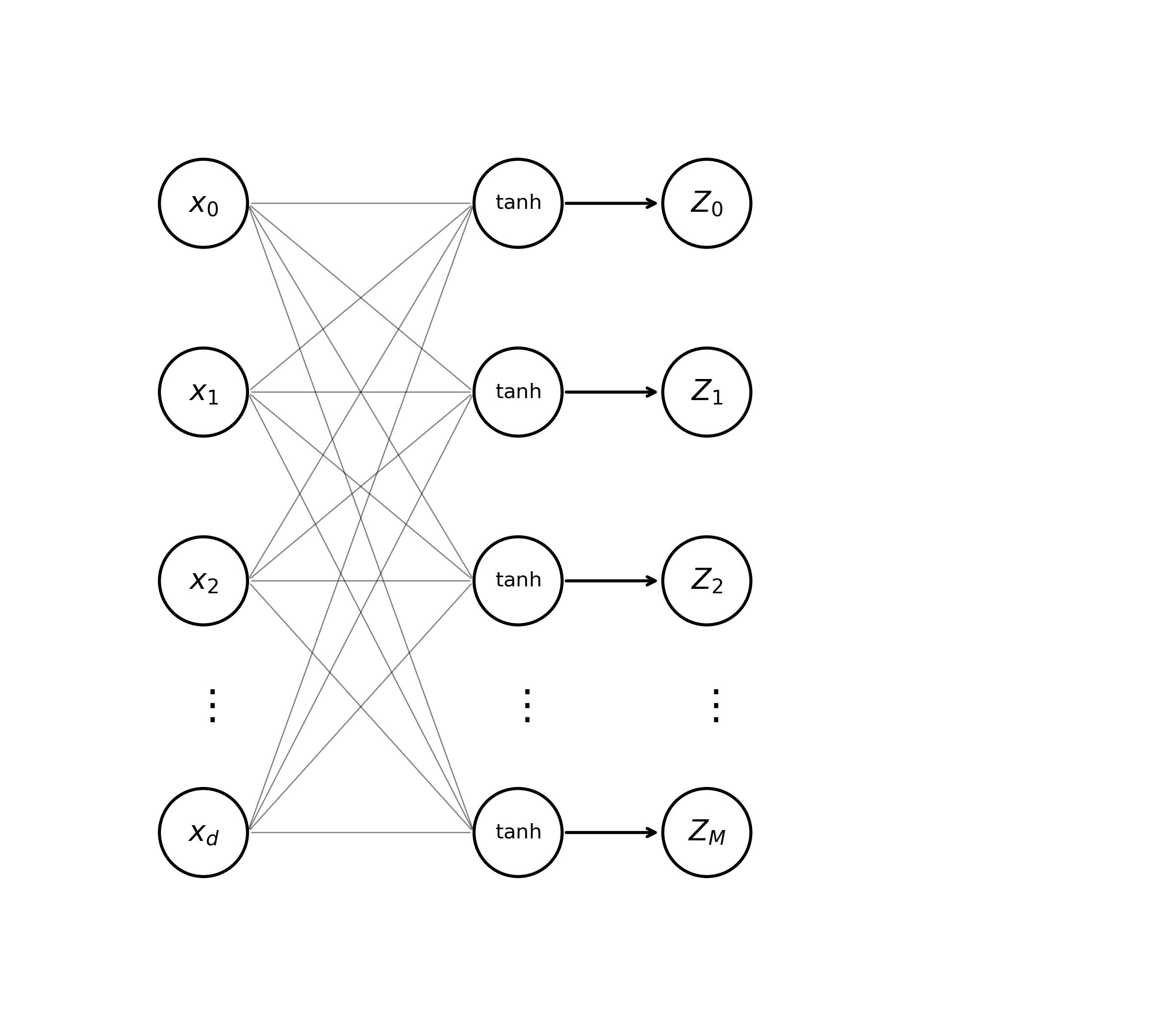
The first and most obvious thing that stands out about this diagram is the density of the connections between the input vector and the hidden state. Just like in our Perceptron, unless they extend to a function, edges in this graph denote multiplication of an input value \(i\) by a weight \(j\): \(w^{( \ell + 1)}_{ji} x_i^{( \ell)}\). To extend this diagram and create an MLP, all we need to do is wire up the hidden state \(\mathbf{z}^{(\ell + 1)}\) to an output vector \(y \in \mathbb{R}^c\). In this second layer, we first calculate values \(\mathbf{a}^{( \ell + 2)} = A^{\top}_{(\ell + 2)} \mathbf{z}^{(\ell + 1)} + b_{(\ell + 2)}\). Finally, we apply a separate non-linear activation function \(\tilde{g}\) to obtain the network output \(y = \tilde{g}(\mathbf{a}^{( \ell + 2)})\). For many applications, such as multiway classification, the softmax function \(\text{softmax}(a_i) = \frac{e^{a_i}}{\sum_{j=1}^{c}e^{a_j}}\), makes a good choice for \(\tilde{g}\).

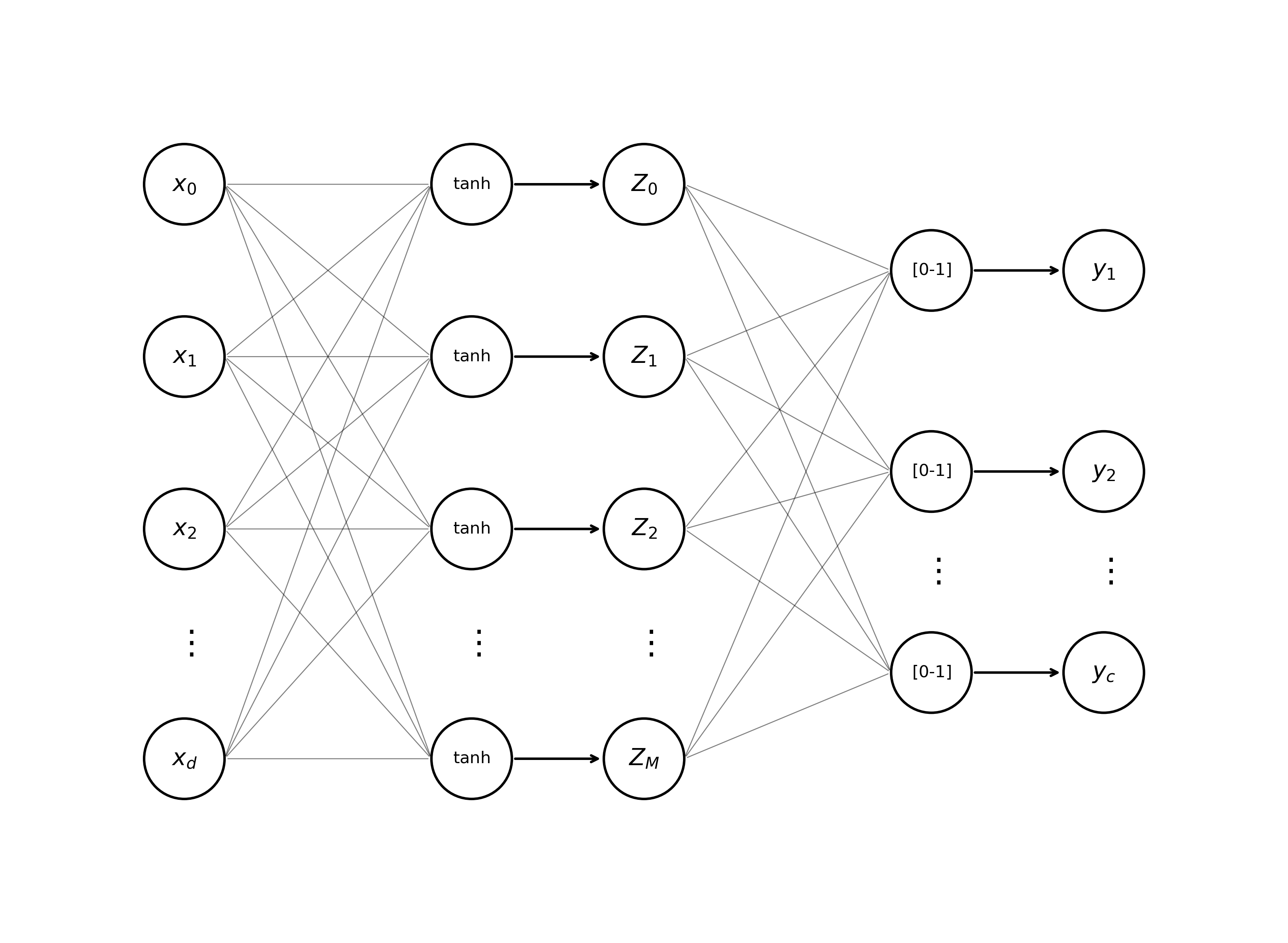
And…we’re done! We’ve just built out our very own Multi-Layer Perceptron! Maybe you’re not excited yet, but you should be! A fully-connected, two-layer neural network like the one above has the power to transform vectors of arbitrary dimensionality to outputs of arbitrary dimensionality, to model simple non-linear functions like “XOR”, and is entirely differentiable–making it well-suited for adaptive learning algorithms like Gradient Descent (which we will be exploring…next week!) Appending just one more layer, that is, expanding our two-layer network into a three-layer network, allows us to learn non-convex (oddly shaped) partitions of any classification space. Consequently, an MLP can solve a much wider range of tasks than a single-unit Perceptron. The extraordinary learning capacities of multi-layered nets become more impressive when you consider that practically any form of data can be represented as a vector.

So we know our model is expressive, but how on earth do you set its weights and thereby help it to reach its full potential? This will be the topic of next week’s ML-Concepts post, where we’re going to dive into Gradient Descent (maybe even SGD if the mood strikes). If you’ve made it this far (god bless you), thank you honestly! There are almost certainly mistakes abound in this post. When you find them, or if you just want to chat, feel free to send me an email.

Thanks for reading!

References

• [1] Bishop, C. M. (1995). The multi-layer perceptron. In Neural networks for pattern recognition (Chapter 4, pp. 116–163). Oxford University Press.