(3/N) Basics of Backpropagation

Back-Propagation Basics

This post is written to be a companion piece to Chapter 4.8 of Christopher Bishop’s seminal textbook: “Neural Networks for Pattern Recognition.” Readers interested in building deeper intuition of the capabilities and limitations of neural networks–as well as the governing mathematics of machine learning–will benefit enormously from a review of this classic treatment.

In our last post, we learned about the expressive power of Multi-Layer Perceptrons (MLPs): feed-forward networks parameterized by weights and bias terms that apply sequential linear transformations to an input vector \(\mathbf{x}\), with non-linear activation functions used at the output of each hidden layer. These remarkable models form an integral part of all modern deep learning architectures. But an MLP with randomly initialized parameters is completely useless to us, regardless of the structure, depth, and topology of the network. To unlock the full potential of these models, we need a general learning algorithm that is applicable to different datasets, runs efficiently on a computer, and learns to update parameters without oversight or instruction.

This brings us to the subject of Back-Propagation: a ubiquitous method for calculating the gradients of a neural network with respect to a loss function. Today, we will outline the high-level concepts and formal mathematics underpinning Back-Propagation. In future posts, this foundation will enable us to analyze more complex solutions to the so-called credit assignment problem, such as those leveraging parallelization or approximations. For now, all we ask is that the reader is familiar with the basics of calculus, particularly gradients of multivariate functions and nested functions.

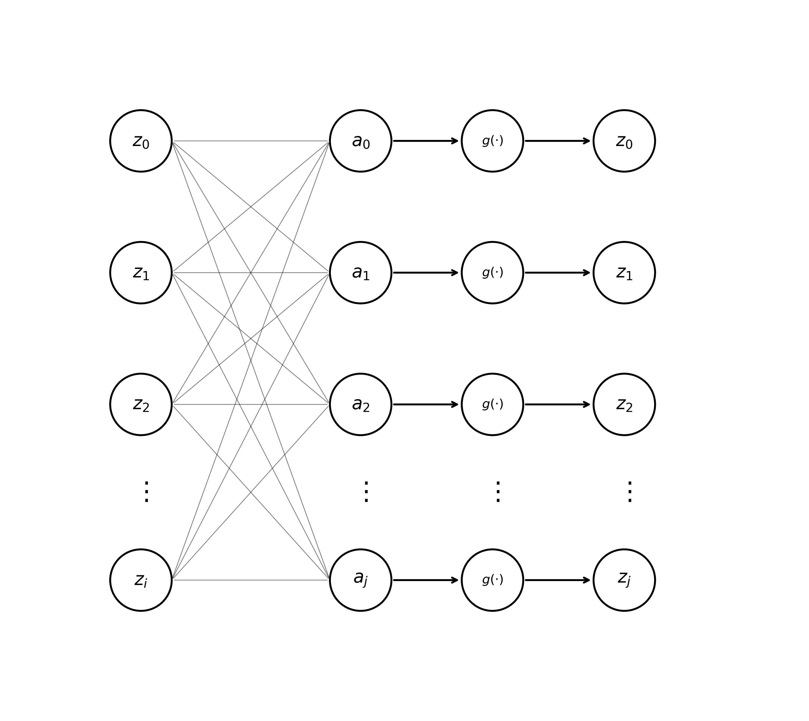
Now, let’s get reacquainted with some notation from previous posts. Recall that a multi-layer net \(\text{MLP}(\mathbf{x}) \mapsto \mathbf{y}\) maps an input vector \(\mathbf{x} = [x_1, x_2, \dots, x_d]\) to an output vector \(\mathbf{y} = [y_1, y_2, \dots, y_k]\). This model is composed of some number of “hidden” layers applied sequentially to the input sequence. For a hidden layer containing \(j\) individual units or “neurons”, the pre-activation \(a_j\) of a unit determined by the previous layer’s activations \(z_i\) can be expressed as

\[\begin{equation} \tag{1} a_j = \sum_i w_{ji}z_i. \end{equation}\]

Here, \(z_i = g(a_i)\), where \(g(\cdot)\) is an activation function (e.g., tanh) and \(b\) is a bias term. In previous posts, we introduced a neat notational trick that allows us to subsume \(b_i\) into a weight vector \(\mathbf{w}\), allowing us to cleanly visualize a hidden layer of an MLP like so.

To set the parameters of any neural network, we first need to formalize the model’s ideal behavior. An error function \(E\) (also referred to as a loss function or objective function) provides a quantitative measure of the quality of a model’s predictions. This function takes the general form \(f: \mathbb{R}^k \mapsto \mathbb{R}\), mapping our model’s output vector \(\mathbf{y}\) to a scalar value typically called a loss. Another way to think of the value \(E\) is as a score that we either want to maximize or minimize depending upon the task at hand. As a concrete example, say our network takes as input Apple’s stock ticker price from a previous week \(\mathbf{x}_{\text{apple}}\), and as output predicts the share prices for the next week \(\mathbf{y}_{\text{pred}}\). We could define a simple sum-of-squares error function for a model, where lower errors indicate better predictions.

\[E_{\text{apple}} = \frac{1}{2}\sum_k (y_k - t_k)^2\]

For reasons that we won’t get into today, the sum-of-squares loss satisfies all the basic criteria required of any error function. Namely, it is convex and differentiable at all points. Importantly, it can be used to steer model behavior in the right direction by punishing incorrect predictions and rewarding outputs closer to the ground truth. Let’s amend our previous visualization of an MLP to include this error function, which is always applied after the activations of the final layer of network are determined.

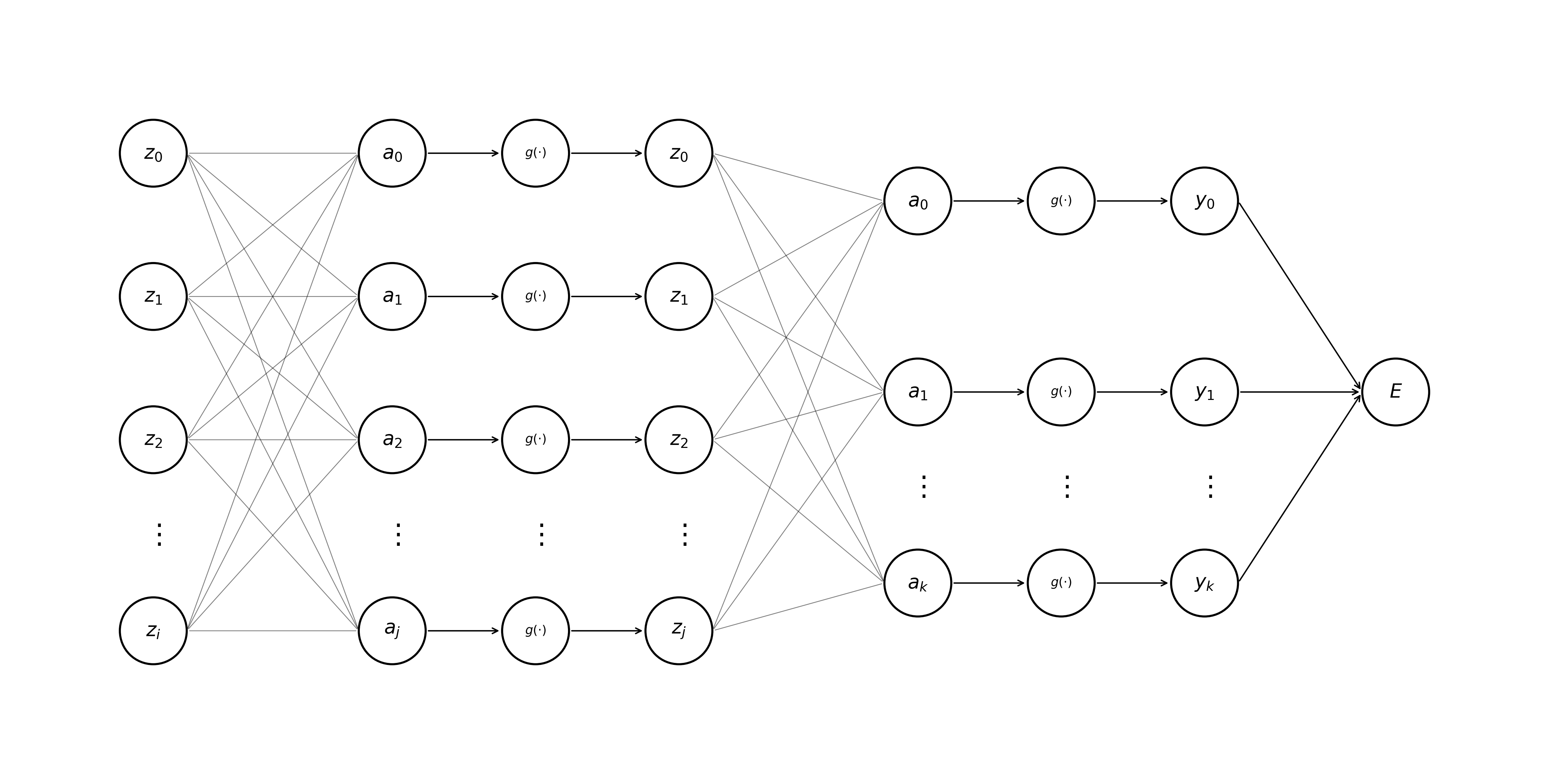
Given some input vector \(\mathbf{x}\), we calculate the forward pass through a neural network \(\text{MLP}(\cdot)\) by applying (Eq. 1) and the formula for the activation of a neuron \(z = g(a)\) sequentially (layer-by-layer). Notice that calculations are computed left-to-right, starting with the hidden layers and terminating with the model’s loss function. The process shown in the animation below is also known as forward propagation.

Now we turn to the problem of credit assignment: the task of computing the contribution of any given weight \(w_{ji}\) with respect to the total error assigned to a model \(E = \sum_{n} E^n\) for a dataset containing \(n\) unique samples. Concretely, we wish to find \(\frac{\partial E^n}{\partial w_{ji}}\) for all parameters in our model. To achieve this, we can leverage the fact that a neural network is essentially a set of nested, differentiable functions. Backpropagation, as the name suggests, is a process that begins at the output (right) of a neural network and works toward the input (left). This procedure makes heavy use of the chain rule; recall from calculus that given a nested function of the form \(y=f(g(x))\), we can find the derivative of the outer function like so.

\[\frac{dy}{dx} = f'(g(x)) \cdot g'(x).\]

Applying the chain rule to our neural network, we can calculate individual weight gradients as the product of the change in error w.r.t. a pre-activation at a hidden unit \(a_j\) and the change in \(a_j\) w.r.t. a model parameter \(w_{ji}\).

\[\begin{equation} \tag{2} \frac{\partial E^n}{\partial w_{ji}} = \frac{\partial E^n}{\partial a_j} \cdot \frac{\partial a_j}{\partial w_{ji}} \end{equation}\]

Before going any further, we’re going to make sure that our understanding of the chain rule is absolutely solid. One way to get a better grasp on this concept as it relates to machine learning is to take a pictorial point of view. All neural nets are really just a big directed acyclic graph, where arrows point from left to right during the forward pass of a model, and right to left during the backward pass (gradient calculation via Back-Propagation). One can intuit that, given an arrow pointing from \(\text{node}_c \rightarrow \text{node}_a\) representing \(\frac{\partial \text{node}_c}{\partial \text{node}_a}\), and another \(\text{node}_{b}\) lying on the path between \(\text{node}_c\) and \(\text{node}_a\), one can visually observe

Or, more formally:

\[\begin{align*} \frac{\partial \text{node}_c}{\partial \text{node}_a} = \frac{\partial \text{node}_c}{\partial \text{node}_b} \cdot \frac{\partial \text{node}_b}{\partial \text{node}_a} \end{align*}.\]

The high-level idea we’re trying to illustrate is that iterative applications of the chain rule allow us to re-use previous computations. In practice, this means that we can implement efficient back-prop algorithms that avoid computing redundant gradients. We’ll now introduce some notation that will become useful later on.

\[\begin{equation} \tag{3} \delta_j \equiv \frac{\partial E^n}{\partial a_j} \end{equation}\]

Here, the value \(\delta_j\) is referred to as the error at a pre-activation \(a_j\). We can also observe that \(\frac{\partial a_j}{\partial w_{ji}} = z_i\). A quick sketch-proof verifies this.

\[\begin{align*} \frac{\partial a_j}{\partial w_{ji}} &= \frac{\partial}{\partial w_{ji}} \Big( \sum_i w_{ji} z_{i} \Big) \\ &= \frac{\partial}{\partial w_{ji}} \Big( \cancel{w_{j0} z_{0}} + \cancel{w_{j1} z_{1}} + \dots + w_{ji} z_{i} \Big) \\ &= z_i \tag*{$\square$} \end{align*}\]

This allows us to rewrite the change in error with respect to the change in a parameter \(w_{ji}\) like so,

\[\begin{equation} \tag{4} \frac{\partial E^n}{\partial w_{ji}} = \delta_j z_i. \end{equation}\]

This is very good news! It turns out that we can re-use the activations of hidden units we calculated during the forward pass in back-prop; all that we need to do is calculate error values \(\delta\) for the hidden and output layers. After this, finding gradients w.r.t. all the weights in our model becomes trivial. To compute the errors of the output layer \(\delta_k\), we can use a slightly different formula than that shown in (Eq. 3),

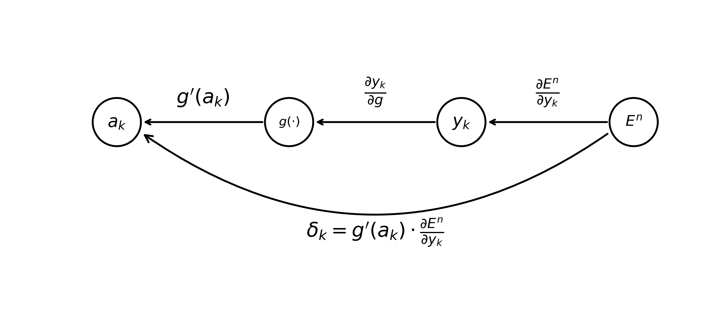
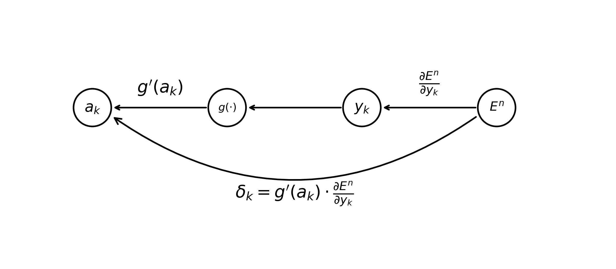
\[\begin{equation} \tag{5} \delta_k \equiv \frac{\partial E^n}{\partial a_k} = g'(a_k) \frac{\partial E^n}{\partial y_k}. \end{equation}\]

As a sanity check, we can show that this statement is true via iterative applications of the chain rule.

\[\begin{align*} \delta_k &= \frac{\partial y_k}{\partial a_k} \frac{\partial E^n}{\partial y_k} \\ &= \frac{\partial g}{\partial a_k} \cancel{ \frac{\partial y_k}{\partial g} } \frac{\partial E^n}{\partial y_k} \\ &= g'(a_k) \frac{\partial E^n}{\partial y_k} \tag*{$\square$} \\ \end{align*}\]

Note that \(\frac{\partial y_k}{\partial g}\) is technically ill-defined; we include this term in the equations above to maintain consistency with the intuition we’ve built up regarding the chain rule. By making this strategic error, we can draw the following diagram.

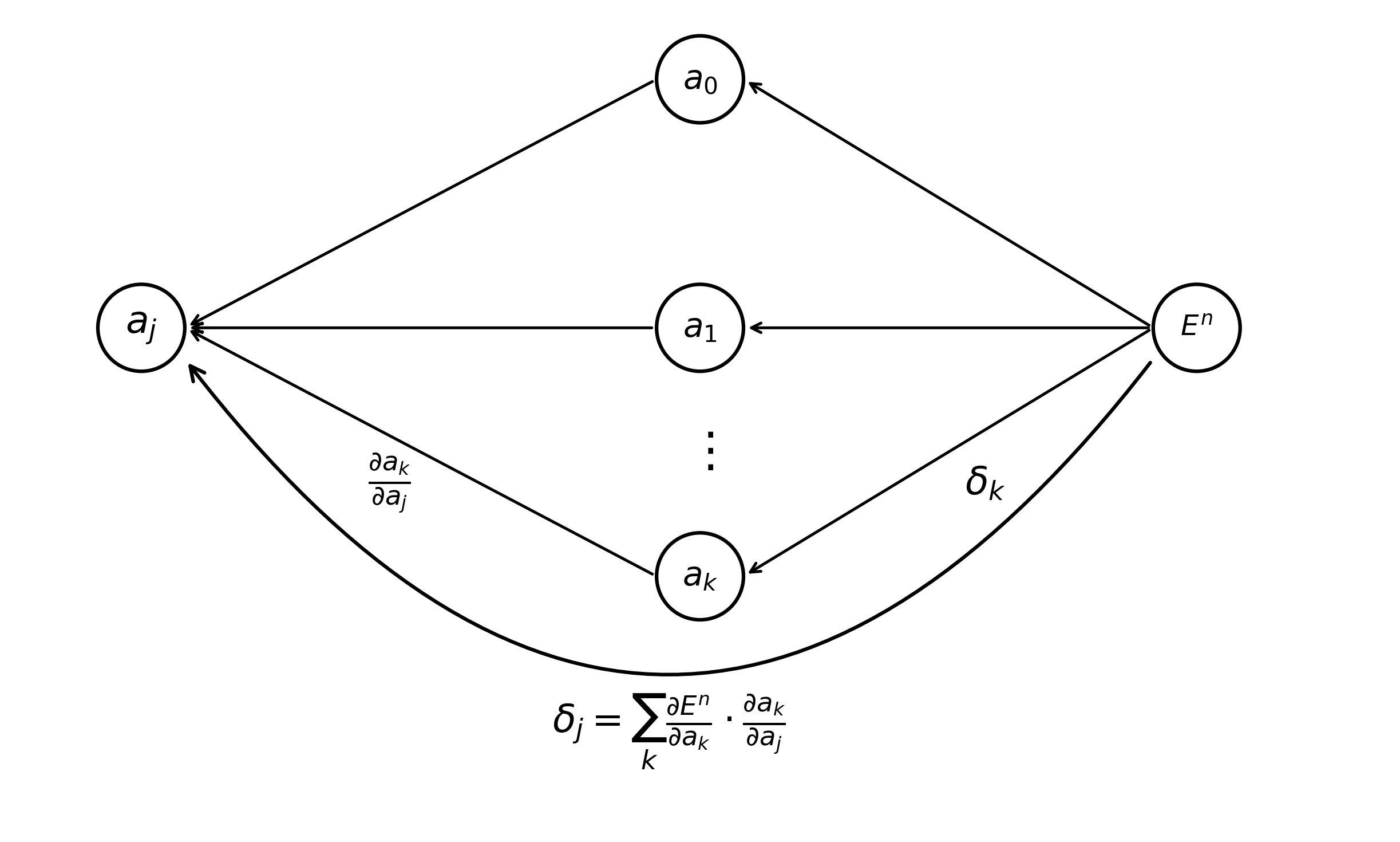
Gradients of pre-activations of our hidden layer \(a_0 \dots a_j\) naturally depend upon all pre-activations in the output layer \(a_0 \dots a_k\). The error of a hidden activation \(\delta_j\) is calculated as a sum of the contribution of each of the pre-activations in the output layer it is connected to. Stated another way, the value of a pre-activation in a hidden layer modulates all units in the output layer.

\[\begin{equation} \tag{6} \delta_j \equiv \frac{\partial E^n}{\partial a_j} = \sum_{k} \frac{\partial E^n}{\partial a_k} \frac{\partial a_k}{\partial a_j} \end{equation}\]

Once again, it is likely a little easier to understand (Eq. 6) using a gradient-flow diagram.

Now we are ready to write out the complete formula for back-propagation. Recall that after completing the forward pass of a model, the only piece of information that we need to calculate any parameter gradient w.r.t. the optimization function \(E\) are the values of \(\delta\) for each unit in our neural network.

\[\begin{equation} \tag{7} \delta_j = g'(a_j) \sum_{k} w_{kj} \delta_k \end{equation}\]

And that’s where we’ll leave things for this week. Back-Propagation is a meaty topic, and it is absolutely imperative that machine learning practitioners understand it deeply to be effective in their field. Next week, we will go over the back-prop algorithm, first in the abstract and next implemented in Python. We’ll also visualize this recursive procedure in action using the figures we’ve built up over the past two weeks. If time permits, we might also explore some efficient variations of the Back-Propagation algorithm.

As always, mistakes, inconsistencies, and omissions are almost certain in these posts. Please bring these items to my attention via my email: levlevi@cs.unc.edu.

Thanks for reading!

References

• [1] Bishop, C. M. (1995). The multi-layer perceptron. In Neural networks for pattern recognition (Chapter 4, pp. 116–163). Oxford University Press.